I have a treat for you today. This blog is probably going to be the most extensive explanation for the Pixel Shuffle layer on the internet. Needless to say, I had fun this week working towards making it so.

Let’s start off with a self-explanatory image to show you what the operation really does.

Now that you understand what the expected output is, let’s look at the simple code needed to produce this.

1
2
3
4
5
6
7
8
9
for n in range(output.size(0)):
  for c in range(output.size(1)):
      for h in range(output.size(2)):
          for w in range(output.size(3)):
              height_idx = h // upscale_factor
              weight_idx = w // upscale_factor
              channel_idx = (upscale_factor * (h % upscale_factor)) + \
                  (w % upscale_factor) + (c * upscale_factor ** 2)
              output[n, c, h, w] = input[n, channel_idx, height_idx, weight_idx]

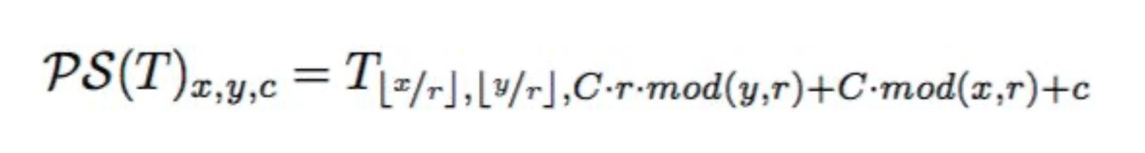
Pretty simple, right? In fact, this is just a translation of the equation from the paper where this layer was born.

I did some more experiments to show you (the audience) and also to understand myself, the working of this layer. The first experiment I did was to only put in non-zero values for a single feature map and zero all the other feature maps to see what the nature of the output is. As you have already seen from the first diagram above, the pixels from each input feature map get mapped to specific pixels in the output feature map. However, if we scale the larger sized output feature map to the same size as the input feature maps and then plot it, then there is very little noticeable difference in the outputs. That is the conclusion I reached from the visualisation below.

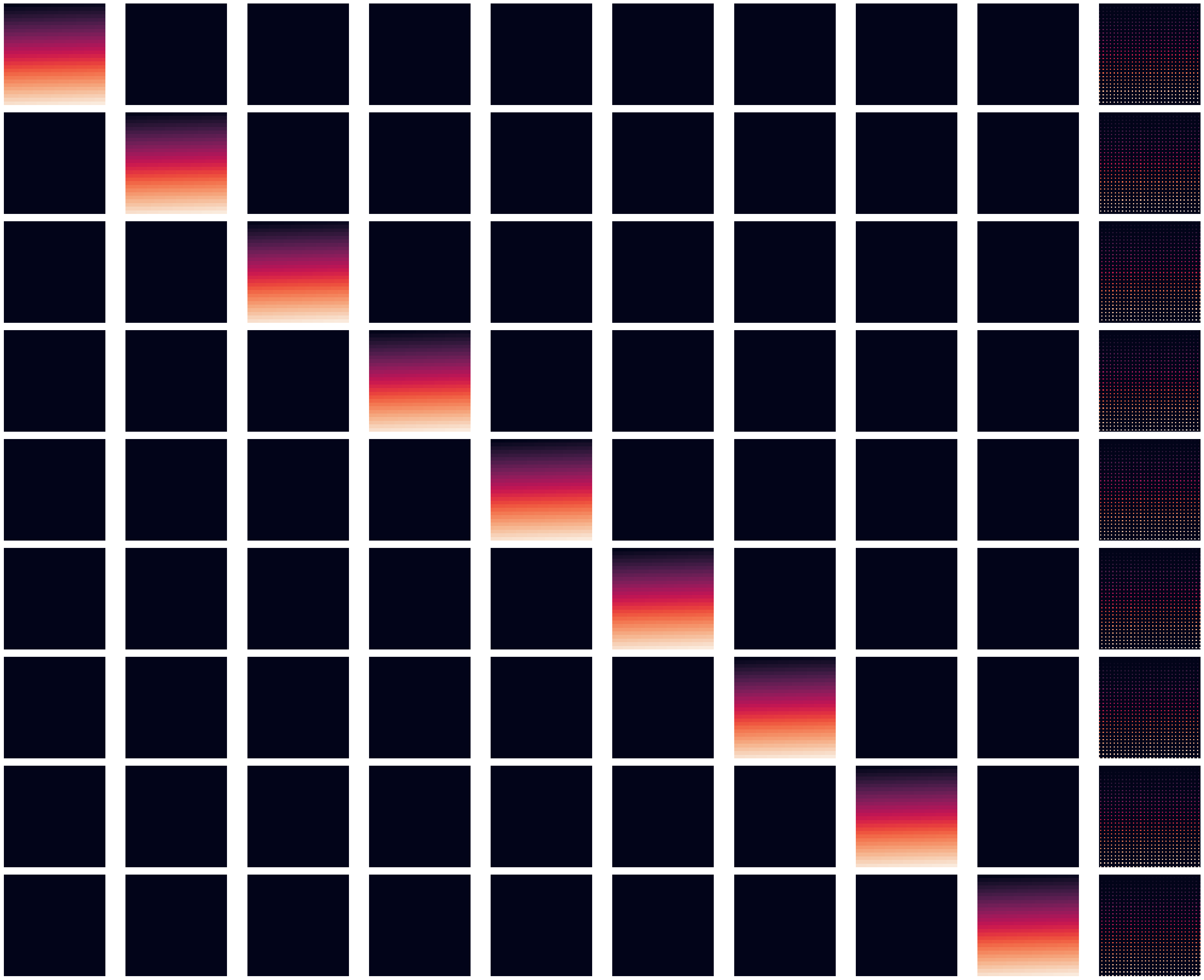
The second experiment I tried out was to apply a sequence of values to 2 feature maps and zero the rest of the feature maps. For this, I generated a linear sequence of numbers from 1 to x, where x is determined using the size of the feature map. In the third experiment, I do the same thing, but apply inverted sequences to the two feature maps. To one of the feature maps, I apply these sequence as input values in increasing order and to another feature map, I apply these in a decreasing order. The idea is, by reversing the orders, the mapping of the pixels should become a bit more apparent than in experiment 1 above. That did indeed happen, with most of the top and bottom pixels of output gaining the higher values corresponding to the higher ends of the series in the inputs. And the middle portion of the output was tending towards black, due to the effect of sparsely distributed lower valued input pixels getting mapped over there. The second and third experiments are visualised with this image, where the colour gradients of the input maps indicate the pixel values present in it.

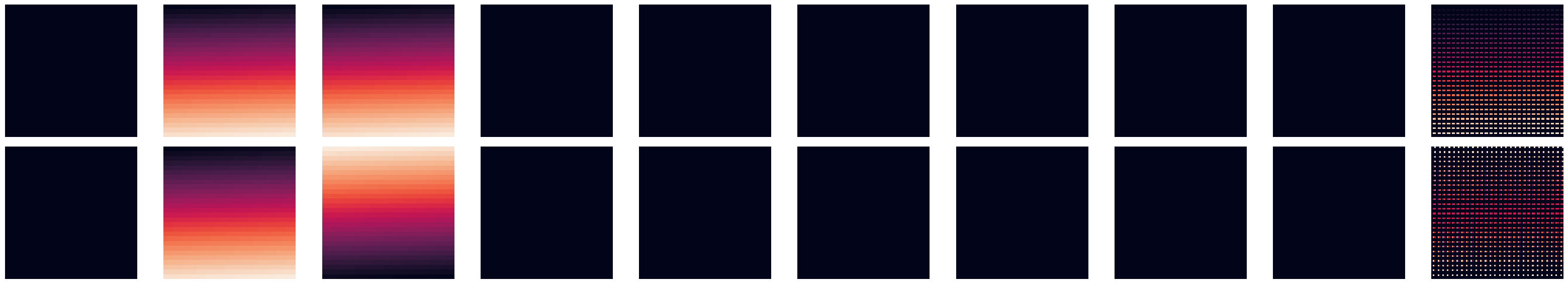
Note that, for all these 3 experiments I considered input shape as (1, 9, 28,28) and output shape as (1, 1, 84, 84). Thus, the first 9 images in each row correspond to the 9 input feature maps each of size 28x28 and the last image is the single output feature map of a larger size 84x84, but plotted to the same size for presenting a clearer visual. Details of all the experiments along with code to reproduce them can be checked from the Google Colab notebook here.

With these visuals done, I had a clearer idea about what the layer was doing and how I should go about approaching the Backward() method of this layer which I was stuck with last week, because PyTorch had implemented it using a complicated 6 dimensional operation.

Initially I was still approaching it incorrectly, thinking that I need to use arma::field() to represent each batch as a cube of cubes, which was not only weird but also doesn’t fit with the rest of the codebase. However, I soon figured out that I could add an extra loop in the layer methods to avoid that unnecessary complication. And, so the Backward() method became really simple to implement. In fact, it can be done just by mirroring the code in the Forward() pass.

1
2
3
4
5
6
7
8
9
for n in range(gy.size(0)):
  for c in range(gy.size(1)):
      for h in range(gy.size(2)):
          for w in range(gy.size(3)):
              height_idx = h // upscale_factor
              weight_idx = w // upscale_factor
              channel_idx = (upscale_factor * (h % upscale_factor)) + \
                  (w % upscale_factor) + (c * upscale_factor ** 2)
              g[n, channel_idx, height_idx, weight_idx] = gy[n, c, h, w]

With that completed, it was only a matter of moments before I could complete the layer along with batch support using an armadillo-only implementation.

The code for matching the PyTorch implementation with the armadillo implementation can be verified from this Google Colab notebook.

All the code related to this layer referred to in this blog post and the previous one can also be found from my github repository, in case any of the Colab links are not working or if I delete those notebooks to save space later on.

That’s it for the Pixel Shuffle layer. I have started looking into the Spatial Dropout layer and will provide further details in the next blog.

Coming to other fun stuff that happened this week, GitHub introduced a cool feature for profile READMEs a few weeks back and I have been enjoying all the cool ideas smart folks have been coming up with. I made my own this week finally and personalising it felt really nice. Almost as if GitHub wants this section of the site to be a place where everyone has some fun.

I also binged the 3rd and final season of the Netflix series Dark, on Friday as usual. Without giving out spoilers, I have to say that the ending they go for makes so much sense giving a feeling of completion to the series, something that makes it magical almost. Here’s a fan-quote punning on one of the iconic dialogues from the series.

Dark is the best Netflix show ever. Never believe anything else.

Music recommendations this week is going to be a bit of K-Pop. Even though I don’t really understand half the lyrics, the songs seem pretty 🔥. I have been binging mainly on BlackPink, but most of the songs I have been hearing aren’t recent ones and I have heard them before. Here is a semi-new one however.

How You Like That by BLACKPINK

See you next week!
XOXO