Convolutional Neural Networks
Project: Write an Algorithm for a Dog Identification App
In this notebook, some template code has already been provided for you, and you will need to implement additional functionality to successfully complete this project. You will not need to modify the included code beyond what is requested. Sections that begin with '(IMPLEMENTATION)' in the header indicate that the following block of code will require additional functionality which you must provide. Instructions will be provided for each section, and the specifics of the implementation are marked in the code block with a 'TODO' statement. Please be sure to read the instructions carefully!
Note: Once you have completed all of the code implementations, you need to finalize your work by exporting the Jupyter Notebook as an HTML document. Before exporting the notebook to html, all of the code cells need to have been run so that reviewers can see the final implementation and output. You can then export the notebook by using the menu above and navigating to File -> Download as -> HTML (.html). Include the finished document along with this notebook as your submission.
In addition to implementing code, there will be questions that you must answer which relate to the project and your implementation. Each section where you will answer a question is preceded by a 'Question X' header. Carefully read each question and provide thorough answers in the following text boxes that begin with 'Answer:'. Your project submission will be evaluated based on your answers to each of the questions and the implementation you provide.
Note: Code and Markdown cells can be executed using the Shift + Enter keyboard shortcut. Markdown cells can be edited by double-clicking the cell to enter edit mode.
The rubric contains optional "Stand Out Suggestions" for enhancing the project beyond the minimum requirements. If you decide to pursue the "Stand Out Suggestions", you should include the code in this Jupyter notebook.
Why We're Here
In this notebook, you will make the first steps towards developing an algorithm that could be used as part of a mobile or web app. At the end of this project, your code will accept any user-supplied image as input. If a dog is detected in the image, it will provide an estimate of the dog's breed. If a human is detected, it will provide an estimate of the dog breed that is most resembling. The image below displays potential sample output of your finished project (... but we expect that each student's algorithm will behave differently!).
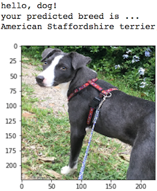
In this real-world setting, you will need to piece together a series of models to perform different tasks; for instance, the algorithm that detects humans in an image will be different from the CNN that infers dog breed. There are many points of possible failure, and no perfect algorithm exists. Your imperfect solution will nonetheless create a fun user experience!
The Road Ahead
We break the notebook into separate steps. Feel free to use the links below to navigate the notebook.
- Step 0: Import Datasets
- Step 1: Detect Humans
- Step 2: Detect Dogs
- Step 3: Create a CNN to Classify Dog Breeds (from Scratch)
- Step 4: Create a CNN to Classify Dog Breeds (using Transfer Learning)
- Step 5: Write your Algorithm
- Step 6: Test Your Algorithm
Step 0: Import Datasets
Make sure that you've downloaded the required human and dog datasets:
Download the dog dataset. Unzip the folder and place it in this project's home directory, at the location
/dog_images.Download the human dataset. Unzip the folder and place it in the home directory, at location
/lfw.
Note: If you are using a Windows machine, you are encouraged to use 7zip to extract the folder.
In the code cell below, we save the file paths for both the human (LFW) dataset and dog dataset in the numpy arrays human_files and dog_files.
import numpy as np
from glob import glob

# load filenames for human and dog images
human_files = np.array(glob("/data/lfw/*/*"))
dog_files = np.array(glob("/data/dog_images/*/*/*"))

# print number of images in each dataset
print('There are %d total human images.' % len(human_files))
print('There are %d total dog images.' % len(dog_files))
Step 1: Detect Humans
In this section, we use OpenCV's implementation of Haar feature-based cascade classifiers to detect human faces in images.
OpenCV provides many pre-trained face detectors, stored as XML files on github. We have downloaded one of these detectors and stored it in the haarcascades directory. In the next code cell, we demonstrate how to use this detector to find human faces in a sample image.
import cv2
import matplotlib.pyplot as plt
%matplotlib inline

# extract pre-trained face detector
face_cascade = cv2.CascadeClassifier('haarcascades/haarcascade_frontalface_alt.xml')

# load color (BGR) image
img = cv2.imread(human_files[0])
# convert BGR image to grayscale
gray = cv2.cvtColor(img, cv2.COLOR_BGR2GRAY)

# find faces in image
faces = face_cascade.detectMultiScale(gray)

# print number of faces detected in the image
print('Number of faces detected:', len(faces))

# get bounding box for each detected face
for (x,y,w,h) in faces:
    # add bounding box to color image
    cv2.rectangle(img,(x,y),(x+w,y+h),(255,0,0),2)

# convert BGR image to RGB for plotting
cv_rgb = cv2.cvtColor(img, cv2.COLOR_BGR2RGB)

# display the image, along with bounding box
plt.imshow(cv_rgb)
plt.show()
Before using any of the face detectors, it is standard procedure to convert the images to grayscale. The detectMultiScale function executes the classifier stored in face_cascade and takes the grayscale image as a parameter.
In the above code, faces is a numpy array of detected faces, where each row corresponds to a detected face. Each detected face is a 1D array with four entries that specifies the bounding box of the detected face. The first two entries in the array (extracted in the above code as x and y) specify the horizontal and vertical positions of the top left corner of the bounding box. The last two entries in the array (extracted here as w and h) specify the width and height of the box.
Write a Human Face Detector
We can use this procedure to write a function that returns True if a human face is detected in an image and False otherwise. This function, aptly named face_detector, takes a string-valued file path to an image as input and appears in the code block below.
# returns "True" if face is detected in image stored at img_path

def face_detector(img_path):
    img = cv2.imread(img_path)
    gray = cv2.cvtColor(img, cv2.COLOR_BGR2GRAY)
    faces = face_cascade.detectMultiScale(gray)
    return len(faces) > 0
(IMPLEMENTATION) Assess the Human Face Detector
Question 1: Use the code cell below to test the performance of the face_detector function.
- What percentage of the first 100 images in
human_fileshave a detected human face? - What percentage of the first 100 images in
dog_fileshave a detected human face?
Ideally, we would like 100% of human images with a detected face and 0% of dog images with a detected face. You will see that our algorithm falls short of this goal, but still gives acceptable performance. We extract the file paths for the first 100 images from each of the datasets and store them in the numpy arrays human_files_short and dog_files_short.
Answer: (You can print out your results and/or write your percentages in this cell)
98% of the first 100 images in human_files have a detected human face.
17% of the first 100 images in dog_files have a detected human face.
from tqdm import tqdm

human_files_short = human_files[:100]
dog_files_short = dog_files[:100]

#-#-# Do NOT modify the code above this line. #-#-#

## TODO: Test the performance of the face_detector algorithm
## on the images in human_files_short and dog_files_short.

count_human_files=0
count_dog_files=0
for img in human_files_short:
    if face_detector(img) :
        count_human_files+=1
for img in dog_files_short:
    if face_detector(img) :
        count_dog_files+=1
print(count_human_files) # 98% of the first 100 images in human_files have a detected human face
print(count_dog_files)   # 17% of the first 100 images in dog_files have a detected human face
We suggest the face detector from OpenCV as a potential way to detect human images in your algorithm, but you are free to explore other approaches, especially approaches that make use of deep learning :). Please use the code cell below to design and test your own face detection algorithm. If you decide to pursue this optional task, report performance on human_files_short and dog_files_short.
### (Optional)
### TODO: Test performance of anotherface detection algorithm.
### Feel free to use as many code cells as needed.
Step 2: Detect Dogs
In this section, we use a pre-trained model to detect dogs in images.
Obtain Pre-trained VGG-16 Model
The code cell below downloads the VGG-16 model, along with weights that have been trained on ImageNet, a very large, very popular dataset used for image classification and other vision tasks. ImageNet contains over 10 million URLs, each linking to an image containing an object from one of 1000 categories.
import torch
import torchvision.models as models

# define VGG16 model
VGG16 = models.vgg16(pretrained=True)

# check if CUDA is available
use_cuda = torch.cuda.is_available()

# move model to GPU if CUDA is available
if use_cuda:
    VGG16 = VGG16.cuda()
Given an image, this pre-trained VGG-16 model returns a prediction (derived from the 1000 possible categories in ImageNet) for the object that is contained in the image.
(IMPLEMENTATION) Making Predictions with a Pre-trained Model
In the next code cell, you will write a function that accepts a path to an image (such as 'dogImages/train/001.Affenpinscher/Affenpinscher_00001.jpg') as input and returns the index corresponding to the ImageNet class that is predicted by the pre-trained VGG-16 model. The output should always be an integer between 0 and 999, inclusive.
Before writing the function, make sure that you take the time to learn how to appropriately pre-process tensors for pre-trained models in the PyTorch documentation.
# check the architecture of the loaded VGG16 Model
VGG16
from PIL import Image
import torchvision.transforms as transforms

def VGG16_predict(img_path):
    '''
    Use pre-trained VGG-16 model to obtain index corresponding to
    predicted ImageNet class for image at specified path

    Args:
        img_path: path to an image

    Returns:
        Index corresponding to VGG-16 model's prediction
    '''

    ## TODO: Complete the function.
    ## Load and pre-process an image from the given img_path
    ## Return the *index* of the predicted class for that image

    ## STEP 1 : Loading the image using PIL.
    loaded_image = Image.open(img_path)
    # plt.imshow(loaded_image)      |
    # plt.show()                    |     These lines are helpful for initial debugging.
    # print(loaded_image.format)    |
    # print(loaded_image.mode)      |
    # print(loaded_image.size)      |

    ## STEP 2 : Pre-processing the image to fit model requirements.
    ## Pre-trained models need normalized 4D tensors with x,y dimensions being atleast 224 pixels,
    ## and also the images have to be RGB. Hence, input shape = [batch_size,3,224,224].
    pre_process = transforms.Compose([  transforms.Resize(256),
                                        transforms.CenterCrop(224),
                                        transforms.ToTensor(),
                                        transforms.Normalize(mean=[0.485, 0.456, 0.406],
                                                             std =[0.229, 0.224, 0.225])])

    input_image = pre_process(loaded_image) # shape is [3,224,224]
    # print(input_image.shape)
    input_image.unsqueeze_(dim=0) # shape is now [1,3,224,224], batch_size=1
    input_image = input_image.cuda()

    ## STEP 3 : Pass the pre-processed image through the model and get output tensor.
    output = VGG16(input_image) # output tensor of size [1,1000].
    # print(output)            |
    # print(output.shape)      |      Helpful for debugging.

    ## STEP 4 : Find the index of the maximum_value in the 1000 columns of output tensor.
    max_val,index = torch.max(output,dim=1)
    # print(max_val)           |
    # print(index)             |    Helpful for debugging
    # print(index.item())      |

    ## STEP 5 : Return the predicted class index as a Python number
    predicted_class_index = index.item()
    return predicted_class_index

    #return #None # predicted class index

# test_img_path = r'images/Brittany_02625.jpg'
# VGG16_predict(test_img_path)
(IMPLEMENTATION) Write a Dog Detector
While looking at the dictionary, you will notice that the categories corresponding to dogs appear in an uninterrupted sequence and correspond to dictionary keys 151-268, inclusive, to include all categories from 'Chihuahua' to 'Mexican hairless'. Thus, in order to check to see if an image is predicted to contain a dog by the pre-trained VGG-16 model, we need only check if the pre-trained model predicts an index between 151 and 268 (inclusive).
Use these ideas to complete the dog_detector function below, which returns True if a dog is detected in an image (and False if not).
### returns "True" if a dog is detected in the image stored at img_path

def dog_detector(img_path):
    ## TODO: Complete the function.
    predicted_index = VGG16_predict(img_path)
    if predicted_index >= 151 and predicted_index <= 268 :
        return True
    return False # true/false

# test_img_path = r'images/Brittany_02625.jpg'
# print(dog_detector(test_img_path))
(IMPLEMENTATION) Assess the Dog Detector
Question 2: Use the code cell below to test the performance of your dog_detector function.
- What percentage of the images in
human_files_shorthave a detected dog? - What percentage of the images in
dog_files_shorthave a detected dog?
Answer:
1% of the first 100 images in human_files have detected a dog in the image.
100% of the first 100 images in dog_files have detected a dog in the image.
### TODO: Test the performance of the dog_detector function
### on the images in human_files_short and dog_files_short.

count_dogs_in_human_files=0
count_dogs_in_dog_files=0
for img in human_files_short:
    if dog_detector(img) :
        count_dogs_in_human_files+=1
for img in dog_files_short:
    if dog_detector(img) :
        count_dogs_in_dog_files+=1
print(count_dogs_in_human_files) # 1% of the first 100 images in human_files have detected a dog in the image.
print(count_dogs_in_dog_files)   # 100% of the first 100 images in dog_files have detected a dog in the image.
We suggest VGG-16 as a potential network to detect dog images in your algorithm, but you are free to explore other pre-trained networks (such as Inception-v3, ResNet-50, etc). Please use the code cell below to test other pre-trained PyTorch models. If you decide to pursue this optional task, report performance on human_files_short and dog_files_short.
### (Optional)
### TODO: Report the performance of another pre-trained network.
### Feel free to use as many code cells as needed.
Step 3: Create a CNN to Classify Dog Breeds (from Scratch)
Now that we have functions for detecting humans and dogs in images, we need a way to predict breed from images. In this step, you will create a CNN that classifies dog breeds. You must create your CNN from scratch (so, you can't use transfer learning yet!), and you must attain a test accuracy of at least 10%. In Step 4 of this notebook, you will have the opportunity to use transfer learning to create a CNN that attains greatly improved accuracy.
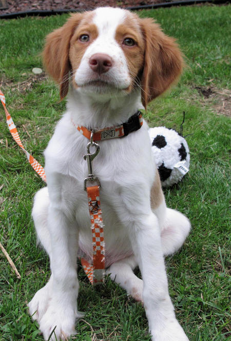
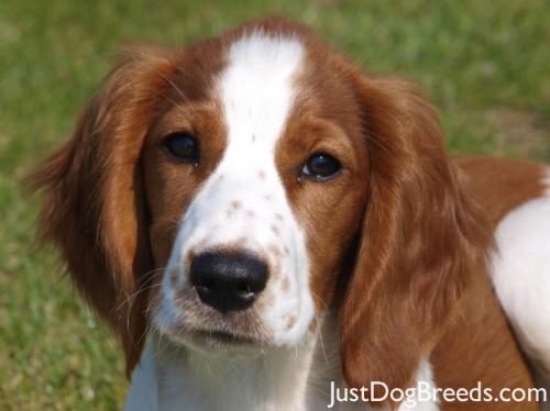
We mention that the task of assigning breed to dogs from images is considered exceptionally challenging. To see why, consider that even a human would have trouble distinguishing between a Brittany and a Welsh Springer Spaniel.
| Brittany | Welsh Springer Spaniel |
|---|---|
 |
 |
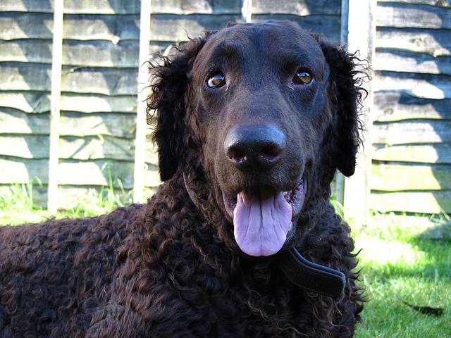
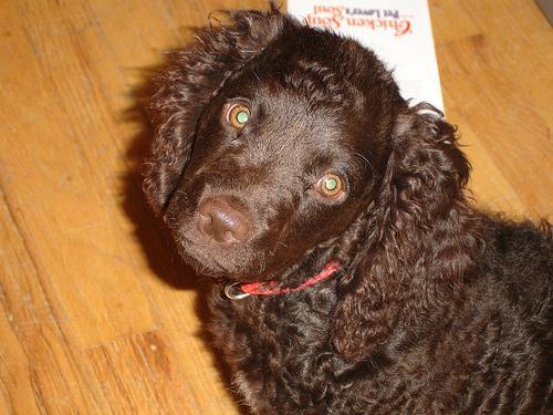
It is not difficult to find other dog breed pairs with minimal inter-class variation (for instance, Curly-Coated Retrievers and American Water Spaniels).
| Curly-Coated Retriever | American Water Spaniel |
|---|---|
 |
 |
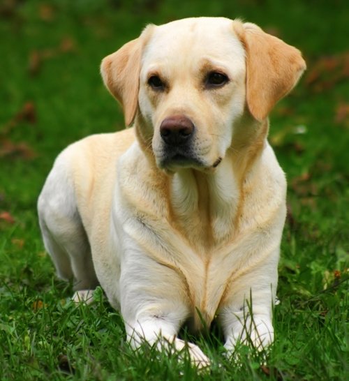
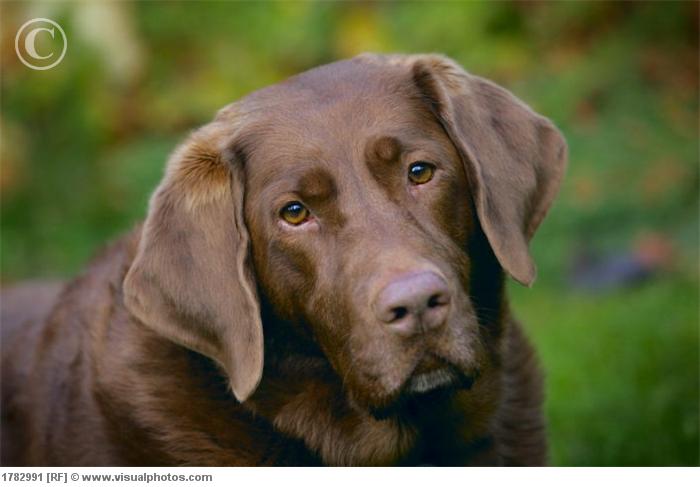
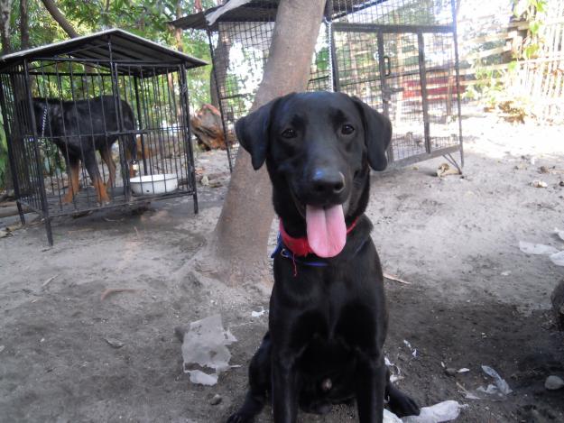
Likewise, recall that labradors come in yellow, chocolate, and black. Your vision-based algorithm will have to conquer this high intra-class variation to determine how to classify all of these different shades as the same breed.
| Yellow Labrador | Chocolate Labrador | Black Labrador |
|---|---|---|
 |
 |
 |
We also mention that random chance presents an exceptionally low bar: setting aside the fact that the classes are slightly imabalanced, a random guess will provide a correct answer roughly 1 in 133 times, which corresponds to an accuracy of less than 1%.
Remember that the practice is far ahead of the theory in deep learning. Experiment with many different architectures, and trust your intuition. And, of course, have fun!
(IMPLEMENTATION) Specify Data Loaders for the Dog Dataset
Use the code cell below to write three separate data loaders for the training, validation, and test datasets of dog images (located at dog_images/train, dog_images/valid, and dog_images/test, respectively). You may find this documentation on custom datasets to be a useful resource. If you are interested in augmenting your training and/or validation data, check out the wide variety of transforms!
import os
from torchvision import datasets
from PIL import ImageFile
ImageFile.LOAD_TRUNCATED_IMAGES = True # necessary to avoid error during training involving loading of truncated bytes of image.

### TODO: Write data loaders for training, validation, and test sets
## Specify appropriate transforms, and batch_sizes

## STEP 1 : Define the different transformations.
train_transforms      = transforms.Compose([transforms.RandomRotation(30),            # rotation invariance
                                            transforms.RandomHorizontalFlip(p=0.6),
                                            transforms.RandomVerticalFlip(p=0.4),
                                            transforms.RandomResizedCrop(224),        # scale invariance
                                            transforms.ToTensor(),
                                            transforms.Normalize([0.485, 0.456, 0.406],
                                                                 [0.229, 0.224, 0.225])])

validation_transforms = transforms.Compose([transforms.Resize(256),
                                            transforms.CenterCrop(224),
                                            transforms.ToTensor(),
                                            transforms.Normalize([0.485, 0.456, 0.406],
                                                                 [0.229, 0.224, 0.225])])

test_transforms       = transforms.Compose([transforms.Resize(256),
                                            transforms.CenterCrop(224),
                                            transforms.ToTensor(),
                                            transforms.Normalize([0.485, 0.456, 0.406],
                                                                 [0.229, 0.224, 0.225])])

## STEP 2 : Get the datasets.
data_dir        = '/data/dog_images'
train_data      = datasets.ImageFolder(data_dir + '/train',
                                       transform=train_transforms)
validation_data = datasets.ImageFolder(data_dir + '/valid',
                                       transform=validation_transforms)
test_data       = datasets.ImageFolder(data_dir + '/test',
                                       transform=test_transforms)

## STEP 3 : Create the DataLoader.
batch_size   = 64
trainLoader  = torch.utils.data.DataLoader(train_data,
                                           batch_size=batch_size,
                                           shuffle=True,
                                           num_workers=0)

validLoader  = torch.utils.data.DataLoader(validation_data,
                                           batch_size=batch_size,
                                           shuffle=True,
                                           num_workers=0)

testLoader  = torch.utils.data.DataLoader(test_data,
                                          batch_size=batch_size,
                                          shuffle=False,
                                          num_workers=0)
# This is needed later on by the train() function
loaders_scratch = {'train' : trainLoader, 'valid' : validLoader,'test' : testLoader}
Question 3: Describe your chosen procedure for preprocessing the data.
- How does your code resize the images (by cropping, stretching, etc)? What size did you pick for the input tensor, and why?
- Did you decide to augment the dataset? If so, how (through translations, flips, rotations, etc)? If not, why not?
Answer :
- transforms.Resize() is used for resizing images to a size that is a power of 2. (256 = 2^8)
- transforms.CenterCrop() is used to crop the images to a size of 224 as it is a standard size used in most models.
- I augmented the dataset with random rotations and horizontal and vertical flips in order to provide rotation invariance.
(IMPLEMENTATION) Model Architecture
Create a CNN to classify dog breed. Use the template in the code cell below.
import torch.nn as nn
import torch.nn.functional as F

# check if CUDA is available
use_cuda = torch.cuda.is_available()

# define the CNN architecture
class Net(nn.Module):
    ### TODO: choose an architecture, and complete the class
    def __init__(self):
        super(Net, self).__init__()
        ## Define layers of a CNN

        # Convolutional Layers                                ##---Dimesionality of input and output channels---##
        self.conv1 = nn.Conv2d(  3 , 64, kernel_size=3, padding=1) # in = [  3,224,224], out = [64,  224, 224]
        self.conv2 = nn.Conv2d( 64, 128, kernel_size=3, padding=1) # in = [ 64,112,112], out = [128, 112, 112]
        self.conv3 = nn.Conv2d(128, 256, kernel_size=3, padding=1) # in = [128, 56, 56], out = [256,  56,  56]
        self.conv4 = nn.Conv2d(256, 512, kernel_size=3, padding=1) # in = [256, 28, 28], out = [512,  28,  28]
        self.conv5 = nn.Conv2d(512, 512, kernel_size=3, padding=1) # in = [512, 14, 14], out = [512,  14,  14]

        # Pooling Layer
        self.pool  = nn.MaxPool2d(2, 2)                            # kernel_size = 2, stride = 2

        # Linear Layers                                      ##---Number of input and output features---##
        self.fc1   = nn.Linear(512*7*7, 512)                       # in = [512*7*7], out = 512
        self.fc2   = nn.Linear(512, 512)                           # in = [512], out = [512]
        self.fc3   = nn.Linear(512, 133)                           # in = [512], out = [133]

        # Dropout Layer
        self.dropout = nn.Dropout(0.5)                             # p = 0.5

    def forward(self, x):
        ## Define forward behavior

        # alternate maxpool and convolutional layers.
        x = self.pool(F.relu(self.conv1(x)))
        x = self.pool(F.relu(self.conv2(x)))
        x = self.pool(F.relu(self.conv3(x)))
        x = self.pool(F.relu(self.conv4(x)))
        x = self.pool(F.relu(self.conv5(x)))

        # Flatten before passing it to the Linear layers.
        x = x.view(-1, 512*7*7)                                     # 512*7*7 = 25088

        # use dropout to prevent overfitting.
        x = F.relu(self.fc1(x))
        x = self.dropout(x)
        x = F.relu(self.fc2(x))
        x = self.dropout(x)
        x = self.fc3(x)

        # return the final output vector of class scores
        return x

#-#-# You do NOT have to modify the code below this line. #-#-#

# instantiate the CNN
model_scratch = Net()

# move tensors to GPU if CUDA is available
if use_cuda:
    model_scratch.cuda()
# check the architecture of the loaded model
model_scratch
Question 4: Outline the steps you took to get to your final CNN architecture and your reasoning at each step.
Answer:
- For the feature extraction part :
I used 5 convolutional layers, all having convolutional kernel of size = 3, stride = 1 and padding = 1, to extract features from the input images.
Convolutional layers are alternated with maxpooling layers of stride=2 and kernel_size=2 to keep the parameters of the network reasonably small, by halving input in size(x,y).This idea is inspired by the VGG architecture.
The depth of the first layer is 3, because the input image has 3 color channels.
The depth of the other layers is chosen as progressively increasing powers of 2.
Kernel size is kept small, as it is known to perform better compared to larger kernels.
- For the classifier part :
The output from the last MaxPool layer is flattened before passing it to the first Linear layer.
3 Linear/Dense layers are used. The last layer has 133 outputs corresponding to the number of classes in the dataset.
Dropout is applied with the probability of 0.5 to reduce overfitting.
- Activation function :
ReLu activation function is used for all the layers of the network. It is preferred over other activation functions because it is sufficiently tolerant to the vanishing gradient problem.
(IMPLEMENTATION) Specify Loss Function and Optimizer
Use the next code cell to specify a loss function and optimizer. Save the chosen loss function as criterion_scratch, and the optimizer as optimizer_scratch below.
import torch.optim as optim

### TODO: select loss function
criterion_scratch = nn.CrossEntropyLoss()

### TODO: select optimizer
optimizer_scratch = optim.Adam(params=model_scratch.parameters(), lr=0.001)
(IMPLEMENTATION) Train and Validate the Model
Train and validate your model in the code cell below. Save the final model parameters at filepath 'model_scratch.pt'.
def train(n_epochs, loaders, model, optimizer, criterion, use_cuda, save_path):
    """returns trained model"""
    # initialize tracker for minimum validation loss
    valid_loss_min = np.Inf

    for epoch in range(1, n_epochs+1):
        # initialize variables to monitor training and validation loss
        train_loss = 0.0
        valid_loss = 0.0

        ###################
        # train the model #
        ###################
        model.train()
        for batch_idx, (data, target) in enumerate(loaders['train']):
            # move to GPU
            if use_cuda:
                data, target = data.cuda(), target.cuda()
            ## find the loss and update the model parameters accordingly
            ## record the average training loss, using something like
            ## train_loss = train_loss + ((1 / (batch_idx + 1)) * (loss.data - train_loss))
            optimizer.zero_grad()
            output = model(data)
            loss = criterion(output,target)
            loss.backward()
            optimizer.step()
            train_loss = train_loss + ((1 / (batch_idx + 1)) * (loss.data - train_loss))

        ######################
        # validate the model #
        ######################
        model.eval()
        for batch_idx, (data, target) in enumerate(loaders['valid']):
            # move to GPU
            if use_cuda:
                data, target = data.cuda(), target.cuda()
            ## update the average validation loss
            output = model(data)
            loss = criterion(output,target)
            valid_loss = valid_loss + ((1 / (batch_idx + 1)) * (loss.data - valid_loss))


        # print training/validation statistics
        print('Epoch: {} \tTraining Loss: {:.6f} \tValidation Loss: {:.6f}'.format(
            epoch,
            train_loss,
            valid_loss
            ))

        ## TODO: save the model if validation loss has decreased
        if valid_loss <= valid_loss_min:
            print('Validation loss decreased ({:.6f} --> {:.6f}).  Saving model ...'.format(
                valid_loss_min,
                valid_loss))
            torch.save(model.state_dict(), save_path)
            valid_loss_min = valid_loss


    # return trained model
    return model


# train the model
model_scratch = train(30, loaders_scratch, model_scratch, optimizer_scratch,
                      criterion_scratch, use_cuda, 'model_scratch.pt')

# load the model that got the best validation accuracy
model_scratch.load_state_dict(torch.load('model_scratch.pt'))
(IMPLEMENTATION) Test the Model
Try out your model on the test dataset of dog images. Use the code cell below to calculate and print the test loss and accuracy. Ensure that your test accuracy is greater than 10%.
def test(loaders, model, criterion, use_cuda):

    # monitor test loss and accuracy
    test_loss = 0.
    correct = 0.
    total = 0.

    model.eval()
    for batch_idx, (data, target) in enumerate(loaders['test']):
        # move to GPU
        if use_cuda:
            data, target = data.cuda(), target.cuda()
        # forward pass: compute predicted outputs by passing inputs to the model
        output = model(data)
        # calculate the loss
        loss = criterion(output, target)
        # update average test loss
        test_loss = test_loss + ((1 / (batch_idx + 1)) * (loss.data - test_loss))
        # convert output probabilities to predicted class
        pred = output.data.max(1, keepdim=True)[1]
        # compare predictions to true label
        correct += np.sum(np.squeeze(pred.eq(target.data.view_as(pred))).cpu().numpy())
        total += data.size(0)

    print('Test Loss: {:.6f}\n'.format(test_loss))

    print('\nTest Accuracy: %2d%% (%2d/%2d)' % (
        100. * correct / total, correct, total))

# call test function
test(loaders_scratch, model_scratch, criterion_scratch, use_cuda)
Results :Test Accuracy came out to be 11% for the model made from scratch. It is just above the minimum threshold requirements for the project.
NOTE : After this point in the Notebook, the kernel was re-started to save GPU time, and hence some of the code from above is copied down below, instead of re-running all the cells above.
Step 4: Create a CNN to Classify Dog Breeds (using Transfer Learning)
You will now use transfer learning to create a CNN that can identify dog breed from images. Your CNN must attain at least 60% accuracy on the test set.
(IMPLEMENTATION) Specify Data Loaders for the Dog Dataset
Use the code cell below to write three separate data loaders for the training, validation, and test datasets of dog images (located at dogImages/train, dogImages/valid, and dogImages/test, respectively).
If you like, you are welcome to use the same data loaders from the previous step, when you created a CNN from scratch.
### Copy pasted all the import and magic statements from above after restarting kernel,
### to avoid running those cells again and waste GPU time in the process.

import numpy as np
from glob import glob
import cv2
import matplotlib.pyplot as plt
%matplotlib inline
from tqdm import tqdm
import torch
import torchvision.models as models
from PIL import Image
import torchvision.transforms as transforms
import os
from torchvision import datasets
from PIL import ImageFile
ImageFile.LOAD_TRUNCATED_IMAGES = True
import torch.nn as nn
import torch.nn.functional as F
import torch.optim as optim
## TODO: Specify data loaders

### Same dataLoader as the previous step is used, with the nly change being in batch_size.
### Previously batch_size was 64 . Now, it is taken as 10.

## STEP 1 : Define the different transformations.
train_transforms      = transforms.Compose([transforms.RandomRotation(30),            # rotation invariance
                                            transforms.RandomHorizontalFlip(p=0.6),
                                            transforms.RandomVerticalFlip(p=0.4),
                                            transforms.RandomResizedCrop(224),        # scale invariance
                                            transforms.ToTensor(),
                                            transforms.Normalize([0.485, 0.456, 0.406],
                                                                 [0.229, 0.224, 0.225])])

validation_transforms = transforms.Compose([transforms.Resize(256),
                                            transforms.CenterCrop(224),
                                            transforms.ToTensor(),
                                            transforms.Normalize([0.485, 0.456, 0.406],
                                                                 [0.229, 0.224, 0.225])])

test_transforms       = transforms.Compose([transforms.Resize(256),
                                            transforms.CenterCrop(224),
                                            transforms.ToTensor(),
                                            transforms.Normalize([0.485, 0.456, 0.406],
                                                                 [0.229, 0.224, 0.225])])

## STEP 2 : Get the datasets.
data_dir        = '/data/dog_images'
train_data      = datasets.ImageFolder(data_dir + '/train',
                                       transform=train_transforms)
validation_data = datasets.ImageFolder(data_dir + '/valid',
                                       transform=validation_transforms)
test_data       = datasets.ImageFolder(data_dir + '/test',
                                       transform=test_transforms)


## STEP 3 : Create the DataLoader.
batch_size  = 10
trainLoader = torch.utils.data.DataLoader(train_data,
                                          batch_size=batch_size,
                                          shuffle=True,
                                          num_workers=0)

validLoader = torch.utils.data.DataLoader(validation_data,
                                          batch_size=batch_size,
                                          shuffle=True,
                                          num_workers=0)

testLoader  = torch.utils.data.DataLoader(test_data,
                                          batch_size=batch_size,
                                          shuffle=False,
                                          num_workers=0)
# This is needed later on by the train() function
loaders_transfer = {'train' : trainLoader, 'valid' : validLoader,'test' : testLoader}
(IMPLEMENTATION) Model Architecture
Use transfer learning to create a CNN to classify dog breed. Use the code cell below, and save your initialized model as the variable model_transfer.
import torchvision.models as models
import torch.nn as nn

## TODO: Specify model architecture

# Used ResNet50 architecture to satisfy minimum accuracy constraints within feasible time.
model_transfer = models.resnet50(pretrained=True)

# check the loaded model architecture
model_transfer
# freeze the parameters
for param in model_transfer.parameters():
    param.requires_grad = False

# modify the output layer
model_transfer.fc = nn.Linear(2048, 133, bias=True)
fc_parameters = model_transfer.fc.parameters()

for param in fc_parameters:
    param.requires_grad = True
# check if CUDA is available
use_cuda = torch.cuda.is_available()

# move model to CUDA if available
if use_cuda:
    model_transfer = model_transfer.cuda()
Question 5: Outline the steps you took to get to your final CNN architecture and your reasoning at each step. Describe why you think the architecture is suitable for the current problem.
Answer:
I tried initially with a VGG architecture. But, it was taking far too long to converge and wasn't giving desired accuracy.
Hence, I decided to switch to ResNet architecture, which usually converges faster. I tried ResNet-152 and ResNet-34 versions, before realizing that they were taking far too long to train or weren't optimal. And finally I settled for the Resnet-50 architecture. It has been pre-trained on ImageNet and hence can detect fine features in images easily enough. Only the final output layer needs to change because in the ImageNet task there are 1000 classes, whereas, here, there are 133 classes.
That is why I chose this particular CNN architecture.
(IMPLEMENTATION) Specify Loss Function and Optimizer
Use the next code cell to specify a loss function and optimizer. Save the chosen loss function as criterion_transfer, and the optimizer as optimizer_transfer below.
criterion_transfer = nn.CrossEntropyLoss()
optimizer_transfer = optim.SGD(model_transfer.fc.parameters(), lr=0.001)
# Adam optimizer was giving comparitively poor performance, hence SGD was used.
(IMPLEMENTATION) Train and Validate the Model
Train and validate your model in the code cell below. Save the final model parameters at filepath 'model_transfer.pt'.
### Copy pasted the train() function from above after restarting kernel,
### to avoid running those cells again and waste GPU time in the process.

def train(n_epochs=10, loaders=loaders_transfer, model=model_transfer,
          optimizer=optimizer_transfer, criterion=criterion_transfer, use_cuda=use_cuda, save_path='model_transfer.pt'):
    """returns trained model"""
    # initialize tracker for minimum validation loss
    valid_loss_min = np.Inf

    for epoch in range(1, n_epochs+1):
        # initialize variables to monitor training and validation loss
        train_loss = 0.0
        valid_loss = 0.0

        ###################
        # train the model #
        ###################
        model.train()
        for batch_idx, (data, target) in enumerate(loaders['train']):
            # move to GPU
            if use_cuda:
                data, target = data.cuda(), target.cuda()
            ## find the loss and update the model parameters accordingly
            ## record the average training loss, using something like
            ## train_loss = train_loss + ((1 / (batch_idx + 1)) * (loss.data - train_loss))
            optimizer.zero_grad()
            output = model(data)
            loss = criterion(output,target)
            loss.backward()
            optimizer.step()
            train_loss = train_loss + ((1 / (batch_idx + 1)) * (loss.data - train_loss))

        ######################
        # validate the model #
        ######################
        model.eval()
        for batch_idx, (data, target) in enumerate(loaders['valid']):
            # move to GPU
            if use_cuda:
                data, target = data.cuda(), target.cuda()
            ## update the average validation loss
            output = model(data)
            loss = criterion(output,target)
            valid_loss = valid_loss + ((1 / (batch_idx + 1)) * (loss.data - valid_loss))


        # print training/validation statistics
        print('Epoch: {} \tTraining Loss: {:.6f} \tValidation Loss: {:.6f}'.format(
            epoch,
            train_loss,
            valid_loss
            ))

        ## TODO: save the model if validation loss has decreased
        if valid_loss <= valid_loss_min:
            print('Validation loss decreased ({:.6f} --> {:.6f}).  Saving model ...'.format(
                valid_loss_min,
                valid_loss))
            torch.save(model.state_dict(), save_path)
            valid_loss_min = valid_loss


    # return trained model
    return model
n_epochs = 10

# train the model
model_transfer = train(n_epochs, loaders_transfer, model_transfer, optimizer_transfer, criterion_transfer, use_cuda, 'model_transfer.pt')

# load the model that got the best validation accuracy (uncomment the line below)
model_transfer.load_state_dict(torch.load('model_transfer.pt'))
# Visualize the different layers in terms of the their sizes.
for param in model_transfer.parameters():
     print(type(param.data), param.size())
(IMPLEMENTATION) Test the Model
Try out your model on the test dataset of dog images. Use the code cell below to calculate and print the test loss and accuracy. Ensure that your test accuracy is greater than 60%.
### Copy pasted the test() function from above after restarting kernel,
### to avoid running those cells again and waste GPU time in the process.

def test(loaders, model, criterion, use_cuda):

    # monitor test loss and accuracy
    test_loss = 0.
    correct = 0.
    total = 0.

    model.eval()
    for batch_idx, (data, target) in enumerate(loaders['test']):
        # move to GPU
        if use_cuda:
            data, target = data.cuda(), target.cuda()
        # forward pass: compute predicted outputs by passing inputs to the model
        output = model(data)
        # calculate the loss
        loss = criterion(output, target)
        # update average test loss
        test_loss = test_loss + ((1 / (batch_idx + 1)) * (loss.data - test_loss))
        # convert output probabilities to predicted class
        pred = output.data.max(1, keepdim=True)[1]
        # compare predictions to true label
        correct += np.sum(np.squeeze(pred.eq(target.data.view_as(pred))).cpu().numpy())
        total += data.size(0)

    print('Test Loss: {:.6f}\n'.format(test_loss))

    print('\nTest Accuracy: %2d%% (%2d/%2d)' % (
        100. * correct / total, correct, total))
test(loaders_transfer, model_transfer, criterion_transfer, use_cuda)
Result : The test accuracy is 62% which is slightly more than the minimum requirement of 60%.
(IMPLEMENTATION) Predict Dog Breed with the Model
Write a function that takes an image path as input and returns the dog breed (Affenpinscher, Afghan hound, etc) that is predicted by your model.
### TODO: Write a function that takes a path to an image as input
### and returns the dog breed that is predicted by the model.
from PIL import Image
import torchvision.transforms as transforms

# list of class names by index, i.e. a name can be accessed like class_names[0]
class_names = [item[4:].replace("_", " ") for item in train_data.classes]

def predict_breed_transfer(img_path):
    # load the image and return the predicted breed

    ## STEP 1 : Loading the image using PIL.
    loaded_image = Image.open(img_path)

    ## STEP 2 : Pre-processing the image to fit model requirements.
    ## Pre-trained models need normalized 4D tensors with x,y dimensions being atleast 224 pixels,
    ## and also the images have to be RGB. Hence, input shape = [batch_size,3,224,224].
    pre_process = transforms.Compose([  transforms.Resize(256),
                                        transforms.CenterCrop(224),
                                        transforms.ToTensor(),
                                        transforms.Normalize(mean=[0.485, 0.456, 0.406],
                                                             std =[0.229, 0.224, 0.225])])
    input_image = pre_process(loaded_image)
    input_image.unsqueeze_(dim=0)
    input_image = input_image.cuda()

    ## STEP 3 : Pass the pre-processed image through the model and get output tensor.
    output = model_transfer(input_image)

    ## STEP 4 : Find the index of the maximum_value in the 1000 columns of output tensor.
    max_val,index = torch.max(output,dim=1)

    ## STEP 5 : Return the predicted class name.
    predicted_class_index = index.item()
    predicted_class_name = class_names[predicted_class_index]

    return predicted_class_name
Step 5: Write your Algorithm
Write an algorithm that accepts a file path to an image and first determines whether the image contains a human, dog, or neither. Then,
- if a dog is detected in the image, return the predicted breed.
- if a human is detected in the image, return the resembling dog breed.
- if neither is detected in the image, provide output that indicates an error.
You are welcome to write your own functions for detecting humans and dogs in images, but feel free to use the face_detector and human_detector functions developed above. You are required to use your CNN from Step 4 to predict dog breed.
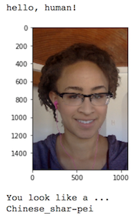
Some sample output for our algorithm is provided below, but feel free to design your own user experience!
(IMPLEMENTATION) Write your Algorithm
Face Detector
### Copy pasted the code for detecting humans from above after restarting kernel,
### to avoid running those cells again and waste GPU time in the process.

face_cascade = cv2.CascadeClassifier('haarcascades/haarcascade_frontalface_alt.xml')
def face_detector(img_path):
    img = cv2.imread(img_path)
    gray = cv2.cvtColor(img, cv2.COLOR_BGR2GRAY)
    faces = face_cascade.detectMultiScale(gray)
    return len(faces) > 0
Dog Detector
### Copy pasted the code for detecting dogs from above after restarting kernel,
### to avoid running those cells again and waste GPU time in the process.

# define VGG16 model
VGG16 = models.vgg16(pretrained=True)

# check if CUDA is available
use_cuda = torch.cuda.is_available()

# move model to GPU if CUDA is available
if use_cuda:
    VGG16 = VGG16.cuda()

def VGG16_predict(img_path):
    ## STEP 1 : Loading the image using PIL
    loaded_image = Image.open(img_path)

    ## STEP 2 : Pre-processing the image to fit model requirements.
    ## Pre-trained models need normalized 4D tensors with x,y dimensions being atleast 224 pixels,
    ## and also the images have to be RGB. Hence, input shape = [batch_size,3,224,224]
    pre_process = transforms.Compose([ transforms.Resize(256),
                                        transforms.CenterCrop(224),
                                        transforms.ToTensor(),
                                        transforms.Normalize(mean=[0.485, 0.456, 0.406],
                                                             std =[0.229, 0.224, 0.225])])

    input_image = pre_process(loaded_image) # shape is [3,224,224]
    input_image.unsqueeze_(dim=0) # shape is now [1,3,224,224], batch_size=1
    input_image = input_image.cuda()

    ## STEP 3 : Pass the pre-processed image through the model and get output tensor.
    output = VGG16(input_image) # output tensor of size [1,1000]

    ## STEP 4 : Find the index of the maximum_value in the 1000 columns of output tensor.
    max_val,index = torch.max(output,dim=1)

    ## STEP 5 : Return the predicted class index as a Python number
    predicted_class_index = index.item()
    return predicted_class_index

def dog_detector(img_path):
    ## TODO: Complete the function.
    predicted_index = VGG16_predict(img_path)
    if predicted_index >= 151 and predicted_index <= 268 :
        return True
    return False # true/false
ALGORITHM :
### TODO: Write your algorithm.
### Feel free to use as many code cells as needed.

def run_app(img_path):
    ## handle cases for a human face, dog, and neither
    loaded_image = Image.open(img_path)
    plt.imshow(loaded_image)
    plt.show()
    if face_detector(img_path):  # Use human face detector defined previously to detect presence of human
        print('You are hereby proven to be a good human being. Congrats !!')
    elif dog_detector(img_path): # Use dog detector defined previously to detect whether dog is present
        print('Woof!Woof!')
        print(predict_breed_transfer(img_path)) # If dog is present, use CNN of step 4 to predict its breed.
    else:
        print('Alien invasion! Alert! You are neither dog nor human!')
Step 6: Test Your Algorithm
In this section, you will take your new algorithm for a spin! What kind of dog does the algorithm think that you look like? If you have a dog, does it predict your dog's breed accurately? If you have a cat, does it mistakenly think that your cat is a dog?
(IMPLEMENTATION) Test Your Algorithm on Sample Images!
Test your algorithm at least six images on your computer. Feel free to use any images you like. Use at least two human and two dog images.
Question 6: Is the output better than you expected :) ? Or worse :( ? Provide at least three possible points of improvement for your algorithm.
Answer: (Three possible points for improvement)
The output is more or less good given the restrictions. It can be improved by some margin as discussed below.
- If in a picture, both dogs and humans are present, algorithm classifies it as neither of the two. This can be improved by training the algorithm a bit differently.
- If there is a very close similarity between two dog species, the algorithm would return only the dominant one. Instead it could be improved, by returning a set of probability scores of the top 3 or top 5 classes.
- Training the underlying CNN on a larger dataset, with more data augmentation and better hyper-parameter tuning could potentially improve the accuracy. Also, adding batch normalization layers would help with the same.
## TODO: Execute your algorithm from Step 6 on
## at least 6 images on your computer.
## Feel free to use as many code cells as needed.

# load filenames for human and dog images
human_files = np.array(glob("/data/lfw/*/*"))
dog_files = np.array(glob("/data/dog_images/*/*/*"))

## suggested code, below
for file in np.hstack((human_files[:3], dog_files[:3])):
    run_app(file)